Here is how we can read it. The probability of the hypothesis (A) given (conditional) on a new piece of evidence (B) is equal to the probability of the evidence (B) given the hypothesis (A) multiplied by the prior probability of the hypothesis (A) divided by the prior probability of the evidence (B).
Ok, let’s stop right here. So I got the following task:
“Write about a topic you are finding particularly challenging. Do it in the form of a tutorial to help another aspiring data scientist to learn that topic.”
Not sure why that is, but probability (P) doesn’t come quickly to me, especially, Bayes’ Theorem. So I made the decision that I would create a blog about it to explain it to myself. If I can do that, it should help others. Now, googling that topic opens a whole world of youtube videos and blogs. Which doesn’t make it any easier.
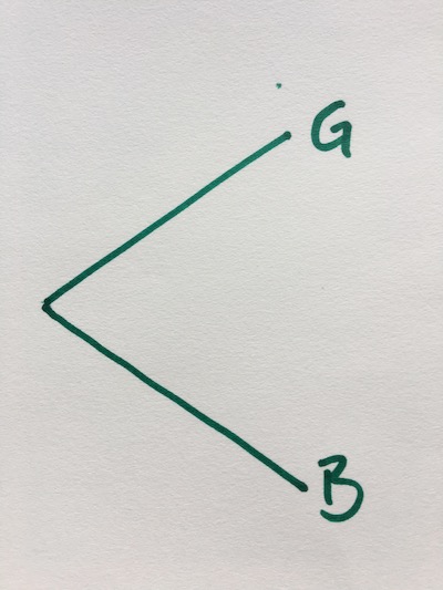
So back to my task. There are several ways to approach Bayes’s Theorem, and the easiest one I found to help me make sense is a tree diagram. To understand the tree diagram for Bayes’ Theorem, let’s demonstrate it on an example. Assume that we have a group of teenagers (girls and boys) and we want to know how many do play soccer. We then would start drawing our tree diagram as follow:
Now depending on how many boys and girls we have in the group we can give each branch some weighting. Let’s say we have a group of 13 girls \(P(G)=0.65\) and 7 boys \(P(B)=0.35\), from which some play soccer \(S\) and others not \(S^c\). To visualize it on our tree diagram we are adding to each branch two more branches.
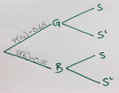
If a teenager plays soccer or not intersects whether or not they are a girl or a boy - denoted as \(P(S \cap B)\) for example. Which brings us to the conditional probability of soccer given it is a boy or a girl, eg. \(P(S∣B)P\). Side note, if we write \(S^c\) to describe the complement of S, we are saying “not playing soccer”.
By adding the new branches, we can view the first two branches as already happened. We are talking about the prior probability of the hypothesis \(P(H)\) and prior probability of the evidence \(P(E)\).
However, before we are moving on, here are two helpful rules to help us solve a given problem.
- all values from each branch have to add up to 1
- we multiply all value going down a branch
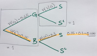
Now, before we can answer any questions, we need some more information, given variables. Like, what is the ratio of girls and boys - which already have from above - and what is the likelihood that a boy or girl plays soccer like so,
\[\large \begin{aligned} P(B) &= 0.35 \small\text{# boys}\\ P(G) &= 0.65 \small\text{# girls} \\ P(S|B) &= 0.3 \small\text{# boys play soccer} \\ P(S|G) &= 0.4 \small\text{# girls play soccer} \end{aligned}\]So with that information, we can solve all our branches. Boys and girls which don’t play soccer, as well as our intersections. Note, that we can write our intersection as \(P(S \cap G)\) or \(P(G \cap S)\), both are the same.
\[\large \begin{aligned} P(S^c | G) &= 0.6 \small\textrm{ # 1 - P(S | G)}\\ P(S^c|B) &= 0.7 \small\textrm{ # 1 - P(S | B)} \\\\ P(S \cap G) &= 0.4 \times 0.65 = 0.24 \\ P(S^c \cap G) &= 0.6 \times 0.65 = 0.39 \\ P(S \cap B) &= 0.3 \times 0.35 = 0.105 \\ P(S^c \cap B) &= 0.7 \times 0.35 = 0.245 \end{aligned}\]Ok, now we can ask questions, for example what is the probability that a girl plays soccer? Or in math terms, \(P(G∣S)\). With the conditional probability rule, we can break this up into
\[\large P(G|S) \rightarrow \frac{P(S \cap G)}{P(S)}\]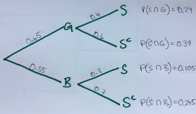
We know what our numerator is by looking at our tree diagram, \(0.24\). For the denumerator however, we need to find out the whole population playings soccer, both boys and girls, and add them together:
\[\large \begin{aligned} P(S) &= P(S \cap B) + P(S \cap G) \\ P(S) &= 0.24 + 0.105 \\ P(S) &= 0.345 \end{aligned}\]So now we can finally solve it:
\[\large \begin{aligned}P(G|S) = \frac{P(S \cap G)}{P(S)} &= \frac{0.24}{0.345} \\\\ P(G|S) &= 0.695 \end{aligned}\]The answer, the probability that a girl plays soccer from that group is 0.695 or 69.5%.
This is Bayes’ Theorem in a nutshell.

